Excel 2013 | Create a unique rule of conditional format
Conditional format that can easily emphasize numerical values.This time, I will introduce how to create and edit the rules of the conditional format.
Create and edit the rules of conditional format
Changing the background color of the cell and the color of the font, displaying graphically with icons and graphs, and conditional format is extremely useful when you want to emphasize the numerical values.Nevertheless, the prepared preset alone does not match the usage scene.
For such a case, the conditional format has a function to create new rules and edit existing rules.The type of conditional format rule, the condition of the change, and the changed format can be combined, and the usage scene is greatly expanded.
Create rules
↑ ↑ ↑ ↑ ↑ ↑ ↑ ↑ ↑ ↑ ↑ 、 、 、 、 、 、 、 、 、 、 変 する 変 する 変 する する する する する するIf the total point exceeds a certain number ...
↑ The background color of the cell changes to yellow.In addition, the color of the font also changes white.The cell that meets the conditions changes automatically.
How to set the rules such as the contents of the change conditions
Creating the rules can be created in a conditional "new rule" of the conditional format.The type of format and conditions of the format can be set arbitrarily.It also supports editing of rules already set.From the "rules management", you can make any changes in conditions and format, as well as corrections of the rules set.
● Step01 Customize the conditions with the “new rules”
↑ First, specify the cell range to set the rules.In drugs, specify the cell you want to be targeted.

↑ Select the “conditional format” of the “home” tab.Select a "new rule" from the developed menu.
● Step02 Select the type of rule and set the change conditions
↑ A mechanism that can be selected and created from 6 types of rules.Here, use the mathematical formula to determine the cell to set the format.
↑ The content of the rules at the bottom changes changes.The box to enter the formula and the preview of the changed format are displayed.
↑ Set mathematical formula in the box with the rules.First, enter the address of the cell to be referenced.Here, enter "= J7".
↑続けて、書式変更の条件を設定。ここでは" >=1600 "と入力し、1600以上の場合に書式を変更するルールを作成。
● Step03 Set the format after the change and complete the creation
↑ Set the format after changing the cells that match the conditions in advance.Select the “Format” button at the right end of the “Preview" item.
↑ In the cell format setting window, first set the background color of the cell."Select the color and select the color.
↑ Continue to set the color of the font.Select the "font tab and select the color to be changed from the list of color" items.
↑ Set the conditions for changing the format, and when the format after the change is determined, click the "button.New rules are completed.
● Step04 Change the contents of the rules already set
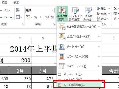
↑ If you want to edit the set rules, select “Rule Management” from the “Conditional Format” menu.
↑ Select the rules you want to change in the rules management window, and select the “edit of the rules” button.
↑ The editing window of the formula rule opens.As in the case of the rule creation, change the type and conditions of the rules.
● Change the scope of the cell with the Step05 rule
↑ Click the reference button on the right side of the "applicable item in the rules management window.
↑ Specify the cell range you want to apply and return to the rules management window.If you select the "OK button ...
↑ The rules under the same condition are applied to the specified cells.For relative reference, the cells to be referenced are also automatically adjusted.


